Different kinds of Fronts
Fronts are areas where two water masses with different properties meet and mix along their boundaries, forming lines in the ocean. The boundaries can be demarcated by differences in water colour, but they are often reflected in changes in temperature, salinity, chlorophyll, sediment load, and in some cases, of density. Temperature fronts, which are also referred to as temperature breaks, are areas where the Sea Surface Temperature (or SST) changes rapidly, creating a gradient in temperature.
Oceanographers distinguish between larger, longer lasting mesoscale fronts and smaller, shorter-lived submesoscale fronts. Mesoscale basically means “middle-sized”. Mesoscale fronts are relatively stable, can last for as long as a season, and sometimes line up along shelf edges or at the edges of major currents or water masses. In contrast, submesoscale fronts are more ephemeral, forming and dissipating with the tides, sometimes lining up at the edges of rips. These smaller fronts can also form part of the surface structure generated by flows past headlands. Fronts may form in the wake of islands that lie in a current stream. Submesoscale fronts can also be entrained (or drawn into) the margins of eddies, which are rotating bodies of water, and they can form along the edges of river-like flows called streamers or jets.
Although I have used a California example in this blog post, the principles are the same wherever fronts occur. In future blogs I will use a New Zealand example to further illustrate these applications of single pass and cloud-free SST imagery to locate promising fishing zones.
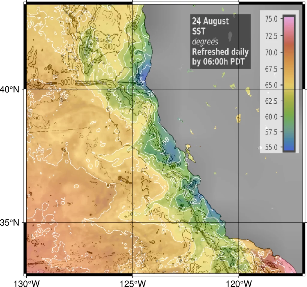
The types of fronts and their characteristics vary by region. Along the coast of central and northern California, mesoscale fronts form at the western edge of cool upwelled water during the summer upwelling season (Figure 1). It’s a relatively stable seasonal feature, and most of the variability is further offshore. Upwelling is initiated by a seasonal change in wind direction, called the Spring Transition, that occurs over a short period at the beginning of spring. The onset of north-west winds blowing parallel to the coast of central California drives surface water offshore, and the surface water is replaced by colder, deeper water, rich in nutrients. The nutrients fuel phytoplankton production, increasing chlorophyll and providing more food for zooplankton. Over a few weeks the coastal upwelling zone develops a food web supporting feed for gamefish like albacore. A frontal boundary persists along the western edge of the upwelling zone where cool upwelled water meets warmer, more offshore waters. The mesoscale fronts at the edge of the upwelling are not transported with the current, and persist for the season.
The zone offshore of the upwelling water is characterised by rivers of offshore transport called streamers. When flows are faster, the streamers are called jets. These streamers and jets transport nutrients, phytoplankton and zooplankton from the productive upwelling nearshore to the less productive offshore waters. Submesoscale fronts form along the edges of these features. Rotating bodies of water called eddies wrap the small scale fronts into their margins. The effect is to create a complex seascape structure of temperature breaks bounding waters with different levels of production. The whole system is anchored to the narrow shelf by the seasonal wind-driven upwelling.
The implications of this structure for game fishing are interesting. In this area, the temperature breaks at the edge of the upwelling are relatively stable and run approximately parallel to the coast. Water is more productive on the cooler, coastal side of the fronts. The breaks further offshore are more complex and variable, running either approximately east-west, or rotating on the edges of eddies. Water is more productive and cooler in the streamers. Albacore exploit these temperature breaks by crossing the breaks to feed in the cool water, and then returning across the front to the warmer water to warm their muscles and increase their swimming speed. This behaviour increases their foraging efficiency. For more detail on albacore behaviour at temperature breaks see my blog called “Albacore tuna and temperature breaks“.
Should I use the most recent SST data, or look for frontal zones, or both?
Fishers often tell me that satellite maps need to be really recent and very high resolution for them to be any use for detecting fronts. As a result, they rely on single pass imagery for the most recent SST. Some fishing app companies tell clients that they process the SST imagery in-house to provide the highest resolution possible, but if they are using the free satellite data from NASA, NOAA and the European Space Agency, the highest resolution (at present) is 0.01 degrees or about 1 kilometer, regardless of whether they process it or not. This is the same resolution that is available as cloud-free SST.
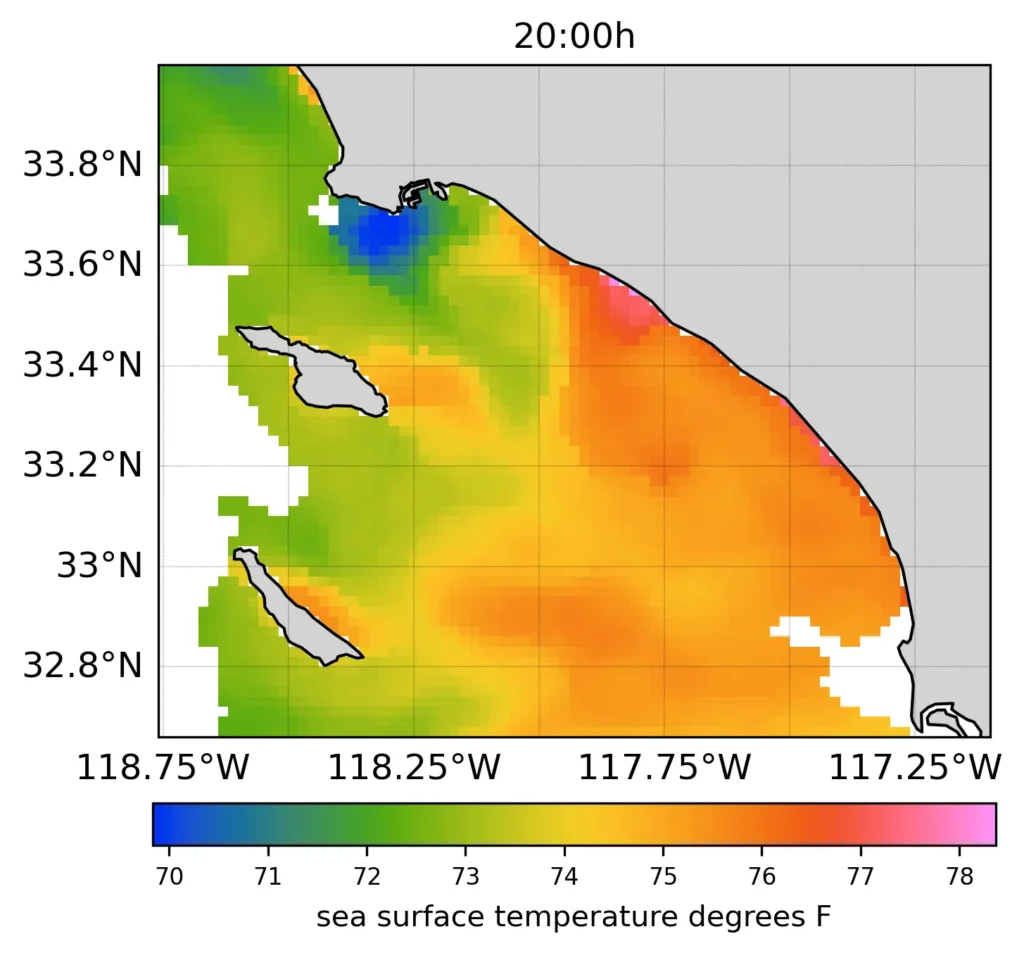
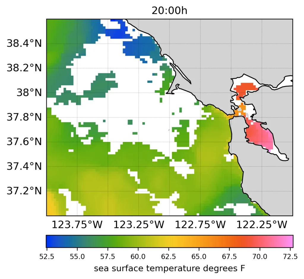
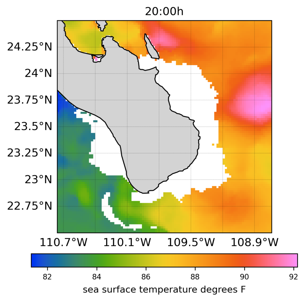
The most recent data from single pass satellite imagery has patchy coverage due to cloud cover. I download 1 kilometer resolution data from a NOAA satellite every 3 hours, but in many cases the patchy coverage prevents determining where the SST front or temperature breaks are. So the most recent satellite maps may not get you very far because of cloud cover, and the resolution will still only be about 1 kilometer. The three maps shown below for Dana Point in southern California (Figure 2), San Francisco in central California (Figure 3), and Cabo San Lucas in Baja Sur (Figure 4) are about as good as single pass imagery gets.
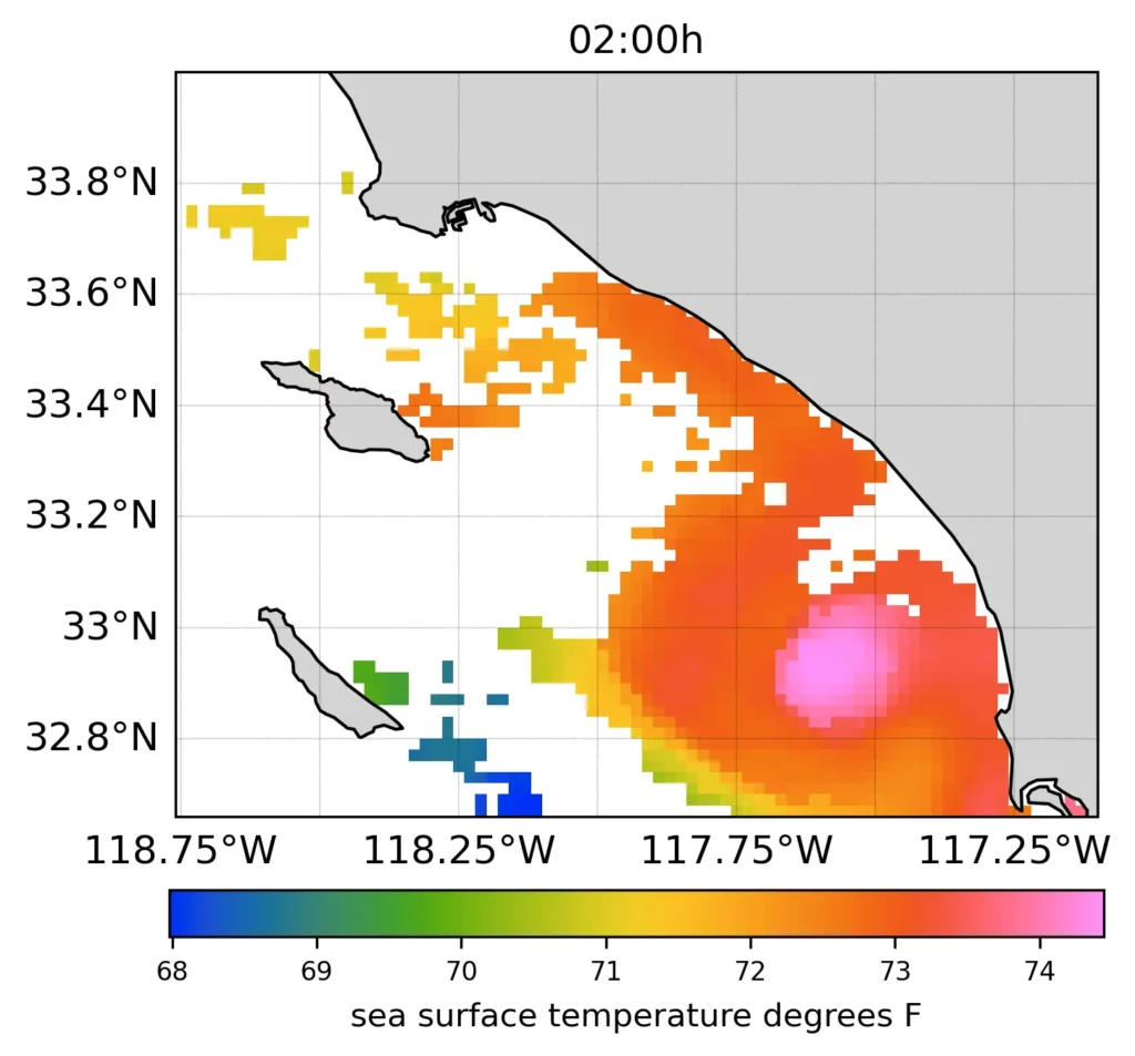
We can compare a single pass SST image for Dana Point, southern California (Figure 5) with four days of cloud-free SST (Figure 6) to illustrate how detecting frontal zones has advantages over using a more recent single pass image. The single pass image shows a patch of 74 degree F water with a 2.5 degree temperature front to the offshore side. This same warm feature is also evident on all 4 days of the cloud-free SST maps, indicating that it was a persistent feature. The temperature front is also clearly defined in the cloud-fee SST by the closely spaced white-coloured temperature contour lines. The 4 cloud-free SST images have several advantages. (1) They show that the feature was persistent over 4 days which is long enough for the plankton and baitfish to respond to small scale flows and nutrient dynamics. (2) They show that the front was more complicated than shown on the single pass image in that the front has both along-shore and cross-shore orientations over a 4 day period. (3) The variability over 4 days defines a frontal zone that can be fished, which is more valuable information than the location of a single temperature break that may form and dissipate, and reform with the tides. This example illustrates the answer to the question “is it better to use the most recent SST data, or to look for frontal zones, or both?” The answer is that both types of information can be combined to determine the best target zone to fish.

Key Points
- Temperature breaks are also called fronts.
- Temperature breaks occur at several scales. This means that temperature breaks can have different sizes (space scales) and can last for varying periods of time (temporal scales).
- Small scale (or submesoscale) fronts are ephemeral or short-lived, often forming and disappearing again with the tidal flows.
- Larger scale (or mesoscale) fronts are much larger, form along persistent features like the shelf edge, and can form and dissipate with the seasons, so they last much longer.
- Targeting the exact position of fronts detected in the most recent satellite images is likely to be less useful than targeting broader frontal zones that persist over several days. This is true because because individual fronts move, within broader frontal zones, and plankton accumulation in frontal zones takes several days to develop.
- Combining the most recent single pass SST images with four days of cloud-free SST imagery provides a good method for locating promising frontal zones to target for game fishing.
- The answer to the question “Is it better to use the most recent SST data, or to look for frontal zones, or both?” is both.